Friday, May 29, 2015

Connector Terminology

Connector gender (Male/Female) for electrical connectors is determined by convention for the given connector, but as expected, the one with the pointier bits compared to it's mating partner is usually designated the male gender.

Jacks, Sockets, Plugs, etc. however, can get a little more complicated.
The terms Jack, Plug, and Socket interpreted in accordance with ASME Y14.44 Reference Designations for Electrical and Electronics Parts and Equipment (plus my own opinion on some others):
  • Jack: A jack is the fixed (or less-movable) connector in a pair, regardless of whether the connector is male/female gender. Reference designator "J" is used in schematic diagrams.
  • Plug: A plug is the moving component of a connector pair, regardless of gender. Reference designator "P" is used. If there are two moving parts such as cables that plug into each other, BOTH connectors can be designated "plugs". Said another way, the plug is the thing you hold in your hand, the jack is the thing you plug into.
  • Socket: Sockets are generally fixed connectors that are used to mount & connect a device or printed circuit directly. Reference designator "X" is used, usually followed by the reference designator of the device it is intended to accept (see the ASME standard for rules for special cases). The distinction between a socket and a jack is that usually jacks are for mating with connectors whereas sockets accept a device package or structure directly (think light-bulb socket which mates directly with the device).
  • Receptacle: Generic term for the electrical contact zone of a female gendered connector - the receiver of a male electrical contact "pin". When describing the number of electrical contacts on a connector, I usually use "N-position pin/receptacle connector."  Sometimes "socket" is used to refer to the individual receptacles.
  • Outlet: Usually used where you have a point where power is being "let out." It is a good idea for power outlets, whether they be jacks or plugs, to be female gendered (having a recessed receptacle) to prevent inadvertent contact with electrically energized surfaces.

Some examples after the break

Thursday, May 21, 2015

Surface Mount Packages Explained

PART 1: Discreet Devices

Surface-mount technology (SMT) discreet devices such as resistors, capacitors, etc. commonly use a four-digit package code such as 0402, 0603, 1206 to indicate their size on datasheets & for ordering. 


SMD capacitor

The two pairs of digits may represent the English units OR MAY represent the rounded unit in tens of mil (milli-inch) for a metric component!

e.g. 0603 may be describing


[06]     [03]
.06"   x .03" 
length   width

when the actual dimensions are 1.6mm x 0.8mm which is .0630" x .0315"


A metric version specification of the same would be 1608M where the pairs of digits represent the number of tenths of a mm. In the US, English style (milli-inches) units is far more prevalent and usually assumed. Always refer to a manufacturer's datasheet for actual device dimensions & tolerances.


Topline has a handly conversion page if you want to know the actual dimensions that correspond to the rounded English-unit description code. 


PART 2: ICs


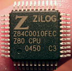
Z84C0010FEC LQFP


Have you seen the terms SOIC, TSOP, SOT23, PLCC, QFP and other alphabet soup in reference to surface mount integrated circuit packages and have trouble keeping them straight? Topline to the rescue again - their SMT nomenclature guide is a nice reference. It describes most surface mount package types for ICs.

Monday, May 18, 2015

LTspice Parameter Stepping Example

LTspice is an excellent SPICE circuit simulation and modeling tool provided free by Linear Technology.

One of the nice features that LTspice provides is the ability to drop SPICE simulation commands right onto your schematic as text - the image after the text illustrates two extremely useful commands: .MEASURE and .STEP

.MEASURE allows you to shortcut the process of using the waveform viewer to painstakingly trace along a waveform for the value you want. The command lets you evaluate a user-customizable expression - key when you want to evaluate the same parameter for a variety of simulation conditions - and will even prepare a table of results if you automate the conditions with .STEP. To see the results (or error messages for malformed commands  ) in LTspice, after simulation open the "SPICE Error Log" (or keyboard shortcut CTRL-L).

LTspice Wiki (unofficial) is a great LTspice resource and includes documentation for the .MEASURE syntax copied from the in-program help (see link for more details):  

Syntax: .MEAS[SURE] [AC|DC|OP|TRAN|TF|NOISE] <name>
 + [<FIND|DERIV|PARAM> <expr>]
 + [WHEN <expr> | AT=<expr>]]
 + [TD=<val1>] [<RISE|FALL|CROSS>=[<count1>|LAST]]

.STEP allows you to automate multiple simulations across a parameter. You can define a generic parameter using .PARAM <name> which can be used as a component value by de-referencing it using {name} and then calculate multiple simulation results/waveforms by sweeping or stepping the parameter. Other things you can "step" include temperature (to look at the temperature effect on your circuit) via parameter temp, model parameters such as transistor width or on-resistance, and even entire part models/subcircuits!

The syntax for .STEP is a little confusing so check out the LT Wiki copy of the in-program help for some examples - 

Syntax: .STEP [OCT|DEC] [<model>|PARAM] <parameter>|<source instance> [LIST] <<start value> <stop value> <steps>>|<list of values>

SPICE commands are activated in LTspice by placing them using the .op tool onto the schematic (Keyboard shortcut 'S').

Below is an example schematic with commands and resulting table of values in the SPICE Error Log. Two different parameters are stepped - temperature and load resistance - and the peak-to-peak difference across the temperature range as well as the average operating point across the temperature range is displayed in the error log. The step numbers correspond to the order specified in the command.


Saturday, May 16, 2015

Coupled Noise Suppression and Brief Overview of Inductive/Capacitive Coupling

I came across a nice illustration (misspellings "chock" aside, haha) of common and differential mode interference and interference suppression. The document concentrates on AC Power Supplies but would be applicable to any signal line.

As a reminder, mutual-inductance indicators ("dots") demonstrate how the common-mode choke suppresses high frequency common-mode currents by generating an opposing/canceling current for each entering line (imagine two equal current pulses both entering in the same direction, each one generating a corresponding pulse through mutual inductance that suppresses the other line's pulse in a kind of cross-cancellation)


High frequency differential noise is shunted across lines by the "X"-style capacitors and high frequency common-mode noise is shunted to chassis/ground by the "Y"-style capacitors (Class X and Y are based on safety capacitors types but I'm using them here to describe their connection configuration).

This document illustrates the difference well.

A discussion on Capacitive (Electric-Field) and Inductive (Magnetic Field) coupling (causes of interference) follows the break. 


Friday, May 8, 2015

Smith Chart and MATLAB Code to Generate

To help me grasp the Smith chart (see Antenna-Theory.com's explanation) I coded up the generation of one in MATLAB. See chart below for illustration of the chart with some explanation and some example moves. 

Code is after the break - it hasn't been cleaned up so apologies for the sparse comments. I used a convenient MATLAB library by Adam Danz for labeling points (labelpoints)

Note that where I say "Constant Reflectance Coefficient" it's technically only the magnitude of the complex value that's constant along the line.


Thursday, May 7, 2015

US Frequency Allocations by NTIA

A fun graphic to see how the radio frequency has been divided in the United States.

A few relevant frequencies (from Wikipedia):
• 4g (cell) - 700 MHz | 750 MHz | 800 MHz | 850 MHz | 1700 MHz | 2100 MHz | 1900 MHz | 2500 MHz
• 3g (cell) - 850 MHz | 1700 MHz | 2100 MHz | 1900 MHz
• 802.11a (WiFi) - 5 GHz | 3.7 GHz
• 802.11b/g (WiFi) - 2.4 GHz
• 802.11n (WiFi) - 2.4 GHz | 5 GHz
• 802.11ac (WiFi) - 5 GHz

Durometer

In engineering, there are a variety of means of quantifying hardness (squishiness) of materials. It's not a straightforward problem because there are many possible dynamics that can come into play with real world materials. Imagine trying to quantify the 'squishiness' of a rubber band versus a pillow versus memory foam - there are many time-dependent factors that greatly complicate things.

A common metric for 'soft' materials is ASTM D2240 Shore Durometer which is a family of tests that gauge the penetration distance of a so-called indentor when a force is applied. The indentors have various specifications for different materials/tests and range from a relatively large diameter (flat-ish) to quite small (sharp-ish).


Common values for some common tests/materials are shown below


For materials that are not so soft (like metals) a similar method to shore durometer is the Rockwell scale where the plastic (permanent) deformation is measured when pressing an indentor into the test material.

By Djhé (Own work) [GFDL (http://www.gnu.org/copyleft/fdl.html) or CC BY-SA 3.0 (http://creativecommons.org/licenses/by-sa/3.0)], via Wikimedia Commons

An alternative for hard objects is the Vickers hardness test which is based on the surface area of indentation of a standard diamond pyramid indentor.

All the above metrics are experimentally determined but provide standard comparative controls for materials.

ASSOCIATED LINKS

Antenna Basics

For a great basic overview on antenna design and basic theory, see Peter Bevelacqua's antenna-theory.com

Digital Signal Processing

For a basic introduction to Fourier Transforms, the theory behind signal decomposing signals into a combination of various single-frequency sinusoidal, I found thefouriertransform.com to be a good overview.


For an excellent, free, practical, and reasonably comprehensive overview of a lot of digital signal topics, see Steve Smith's online textbook (downloadable for personal use).
Topics include
* Sampling theory/fundamentals
* Analog to digital and digital to analog conversion
* Convolution and Fourier Transforms
* Digital Filters
* Various Applications examples
* Further advanced mathematics (e.g. Laplace transform, z-transform)
For most algorithm discussions (FFT etc.), he includes code (sadly it's BASIC) to illustrate, a nice touch.

Wednesday, May 6, 2015

MATLAB Quick Reference and Function/Class Templates

%%%%%%%%%%%%%%%%%%%%%%%%%%%%%%%%%%%%%%%%%%%%%%%%%%%%%%%
% MATLAB QUICK REFERENCE AND FUNCTION/CLASS TEMPLATES %
%%%%%%%%%%%%%%%%%%%%%%%%%%%%%%%%%%%%%%%%%%%%%%%%%%%%%%%

%%%%%%%%%%%%%%%%%%%%%%%%%%%%%%%%%
% INDEXING & MATRIX REFERENCING %
%%%%%%%%%%%%%%%%%%%%%%%%%%%%%%%%%

% NOTE: Matlab uses indexing that starts at 1, not 0

a';     % Transpose vector/matrix 'a'
a(1);       % Return first element of vector 'a'
a(1,:);     % Return first row of matrix 'a' (all columns)
a(:,1);     % Return first column of matrix 'a' (all rows)
a(i:j:end); % Extract every jth value starting at i until the last value
% Note: 'end' keyword can be used to refer to last index without using size() method
a(1:5, 10:20)   % Return matrix rows 1 through 5 and columns 10 through 20 of 'a'

[r,c]=size(a);  % Find number of rows & columns in matrix 'a'
length(a);      % Length of vector 'a'
size(a,d);      % Find length of 'd'th dimension, e.g. 1=rows,2=columns,3=z
find(a > 1);    % Returns list of indexes in 'a' whose value is >1. Can use any logical e.g. a=1
[r,c]=find(a);  % Returns list of all indexes with nonzero values, in this case row/col index pairs from a 2-D matrix

zeros(r,c); % Creates a r-rows by c-columns matrix of zeros
ones(r,c);  % Creates a r-rows by c-columns matrix of ones
rand(r,c);  % Creates a r-rows by c-columns matrix of pseudo-random numbers from the 0-1 scale (uniform dist)

%%%%%%%%%
% Spans %
%%%%%%%%%

linspace(a,b,n);    % Creates a row vector that spans 'a' to 'b' in 'n' number of linearly spaced segments
logspace(a,b,n);    % Creates a row vector that spans 10^a to 10^b in 'n' points
x=a:n:b;            % Creates a row vector from 'a' to 'b' spaced by value 'n'
repmat(A,r,c);      % Tile matrix A 'r' times in the rows direction, 'c' times in the cols direction
flip(A,<dim>);      % Flip order of a vector/matrix, optionally along a specified dimension
horzcat(A,B);       % Horizontally concatenate vectors/matricies A, B, C, D, etc.
vertcat(A,B);       % Vertically concatenante vectors/matricies A,B,C,D, etc.

%%%%%%%%%%%
% FIGURES %
%%%%%%%%%%%

close all% Close all open figures
figure;     % Create new figure
figure(1);  % Select given figure and make it active, or create one with given handle
subplot(numRows,numCols,selectActivePlotNum); % Create framework for multiple plots within one figure and/or select one

plot(x,y,<LineSpec>);   % X values, corresponding Y values, LineSpec optional
% LineSpec is a string composed of concatenating the following specifiers e.g. '--xc'
% Note: LineSpec with Marker but no Style will plot only markers without a line
% Styles: '-'Solid | '--'Dashed | ':'Dotted | '-.'Dash-Dot
% Markers: 'o' '+' '*' '.' 'x'  's'square 'd'diamond '^'triangle 'v'triangle & others...
% Colors: 'y'yellow | 'm'magenta | 'c'cyan | 'r'red | 'g'green | 'b'blue | 'w'white | 'k'black

stem(x,y);  % Plot discrete sequence data
hist(data,<nbins>); % Plot histogram of 10 equally spaced bins, or bins as specified
histfit(data,<nbins>,<distToFit>);  % Plot histogram with best-fit distribution
normplot(data); % Normal probability plot i.e. normal quantile plot

gcf;    % 'Get Current Figure' Returns handle/reference to active figure
gca;    % 'Get Current Axis' Returns handle/reference to active axis

% Note: for one-time plots it can be easier to format using Show Plot Tools in menubar
% Note: TeX markup can be used in strings
% Note: Formatting/plot commands are applied to the currently active figure
title({'Main Title Here';'\fontsize{8}Smaller Subtitle Here'});
xlabel('X Axis Units');
ylabel('Y Axis Units');
xlim([xmin xmax]);  % Manually set X limits for plot
ylim([ymin ymax]);  % Manually set Y limits for plot

saveas(gcf,'figure.png');   % Save figure as image


%%%%%%%%%%%%%%%%%%%%%%%%%%%%%
% Loops and Logical Control %
%%%%%%%%%%%%%%%%%%%%%%%%%%%%%

for i=1:n:10    % for(i=1;i<=10;i+=n)
    % Do Things
end

if <logical statement>
    % Do Things
elseif <logical statement>
    % Do Things
else
    % Do Things
end

%%%%%%%%%%%%%%%%%%%%%%%%%%%%%%
% Curve Fitting & Regression %
%%%%%%%%%%%%%%%%%%%%%%%%%%%%%%

fitobject = fit(x,y,fitType);   % REFER TO MATLAB HELP/DOCUMENTATION for details - Curve Fitting Toolbox
plot(fitobject,x,y,{'fit','residuals','deriv1'}); % Plot fit along with input data, as well as residuals vs. fit and 1st derivative

%%%%%%%%%%%%%
% FUNCTIONS %
%%%%%%%%%%%%%

% Note: Main function names and corresponding filenames should match.
% Note: Any additional functions in an m-file beyond the first/main function
% are 'local functions' with calling scope limited to the main function
function [returnA, returnB] = functionName(inputA, inputB, varargin)
    %functionName(inputA, inputB, <variable number of arguments>)
    %   Detailed explanation here

    n=nargin; % Number of input arguments
end

%%%%%%%%%%%
% CLASSES %
%%%%%%%%%%%

classdef exampleClass < handle      % Inheriting from handle is necessary to be able to refer to class instance
    %EXAMPLECLASS Summary of this class goes here
    %   Detailed explanation goes here
   
    properties
        Data;
    end
   
    methods
        function obj=exampleClass(input)    % Constructor
            obj.Data=input;
        end

        function []=methodOne(obj,inputArg)
            % This function would be called by exampleClass.methodOne(inputArg)
            % The first argument is a reference/handle to the class instance       
            % This function does not return a value

            obj.Data=inputArg;  % This type of statement will change the class instance's variable value
        end
    end
end

%%%%%%%%%
% OTHER %
%%%%%%%%%

% NOTE: any statement without a trailing semi-colon will display the result in the command window

% General suggestions
% • Use the workspace variable explorer when creating complex matrixes to visually validate your code is creating what you expect regarding dimensions etc.
% • Make liberal use of the debugger and the capability to perform commands in the Command Window and see workspace variables DURING debugging to explore what your code is doing

% Keyboard Shortcuts:
% • Ctrl-R comments line(s)
% • Ctrl-T un-comments line(s)
% • Tab to indent line(s) (select multiple if desired)
% • Shift-Tab to de-indent line(s) (select multiple if desired)

clear;      % Delete/destroy workspace variables
clc;        % Clear command window
isempty(A); % Check whether variable A is an empty array

fprintf('String %.1d \n',value);    % Print strings and values to cons

-----------------------------------------------

ASSOCIATED LINKS

Friday, May 1, 2015

Technical and Math Character Entry

Some technical "alt-character" shortcuts I find useful are below. I've memorized some favorites like • and Ω. List bullet symbol entry is particularly useful for lists in software that doesn't traditionally support them, such as within Excel cells or in basic text editors.

Another quick tip is to use "ALT =" in most Microsoft products (Word, OneNote) to quickly enter the "formula-entry" mode.

In this mode, most special characters can be entered using LaTeX syntax. Here's a decent cheat sheet for LaTeX codes for math symbols.

HOW TO:
Enter a character by holding "ALT" key and typing out the numeric (note leading zeros) on the keyboard Numpad.

Some alternative means for character entry:
  • Copy-paste the characters from this webpage
  • Windows "Character Map" program (on Windows 7+ search start-menu for Character Map)
  • In many Microsoft products (Word, Outlook), Alt-"=" (no quotes) will start the equation editor
  • Google-search a description of the character you want, copy and paste from search results
-----------------------------------
MY FAVORITES:
• | Alt-0149 | List Bullet
Ω | Alt-234 | Omega (uppercase) (Ohms)
σ | Alt-229 | Sigma (lowercase) (standard deviation)
µ | Alt-230 | Mu (lowercase) (mean)
± | Alt-0177 | Plus/Minus (bilateral tolerancing, uncertainty)
≈ | Alt-247 | Approximately equal to
° | Alt-0176 | Degrees

GENERAL
• | Alt-0149 | List Bullet
§ | Alt-0167 | Section symbol
↑ | Alt-24 | Up Arrow
↓ | Alt-25 | Down Arrow
→ | Alt-26 | Right Arrow
← | Alt-27 | Left Arrow

MATH SYMBOLS
± | Alt-0177 | Plus/Minus
÷ | Alt-0247 | Division
° | Alt-0176 | Degrees
≥ | Alt-242 | Greater than or equal to
≤ | Alt-243 | Less than or equal to
≈ | Alt-247 | Approximately equal to
× | Alt-0215 | Multiplication (alternate)
¬ | Alt-0172 | Boolean Algebra “Not”
√ | Alt-251 | Square Root
² | Alt-0178 | Squared
³ | Alt-0179 | Cubed
 | Alt-193 | Perpendicular
∩ | Alt-239 | Intersection

GREEK LETTERS
α | Alt-224 | Alpha (lowercase)
ß | Alt-225 | Beta (lowercase)
Γ | Alt-226 | Gamma (lowercase)
π | Alt-227 | Pi (lowercase)
Σ | Alt-228 | Sigma (uppercase)
σ | Alt-229 | Sigma (lowercase)
µ | Alt-230 | Mu (lowercase)
τ | Alt-231 | Tau (lowercase)
Φ | Alt-232 | Phi (uppercase)
Θ | Alt-233 | Theta (uppercase)
Ω | Alt-234 | Omega (uppercase)
δ | Alt-235 | Delta (lowercase)
φ | Alt-237 | Phi (lowercase)
ε | Alt-238 | Epsilon (lowercase)
-----------------------------------

ASSOCIATED LINKS
ASCII
Unicode
Greek Letters used in Math, Science, & Engineering